I live in the Western United States. I’ll occasionally see a sign when I’m driving that says, “Open Range Area.” It means I must look out for wandering animals. Rather than putting up fences to prevent the carnage of an accident, we put up signs and hope for the best.
It’s easy to create an inaccurate CVP analysis that lacks signs to warn us that we’ve gone past the boundaries of what’s called the relevant range. There can be serious business carnage when we wander beyond that range.
The Relevant Range
Here is a classic Cost-Volume-Profit (CVP) line graph.
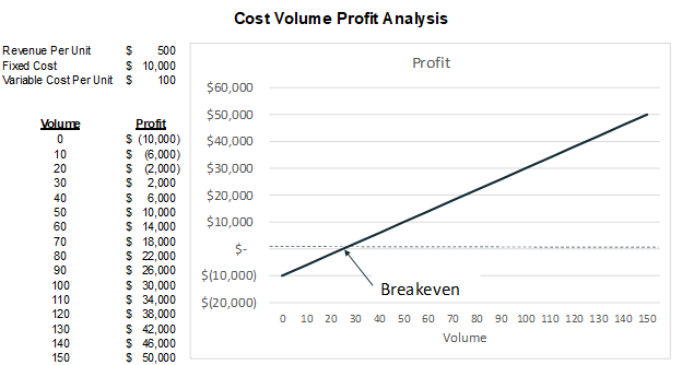
Some assumptions must be true for this line to be completely straight. These assumptions include:
- The price per unit does not change
- Fixed costs do not change
- The variable cost per unit does not change
The range of volume for which these statements are assumed to be true is called the relevant range. A CVP or break-even analysis is only correct for the relevant range in which its assumptions are valid.
What could cause these assumptions to be invalid? More specifically, what could cause the price and costs to change?
Price per Unit
What’s the easiest way to increase sales volume? Lower the price per unit. Conversely, sales unit volumes often decrease when you raise the price of a product. So, if an analysis says that the break-even point is higher than the current volumes, how do you increase sales volumes without lowering the price? Once you lower the price to increase volumes, the break-even point goes up, which may mean you need to lower the price even more. This can create an analysis spiral. Thinking of additional advertising to increase sales? That also raises fixed or variable costs and increases the break-even point.
Variable Costs
Variable costs can increase or decrease at higher volumes. Raw materials and parts can often be obtained at lower per-unit costs when purchased in bulk. There may be other economies of scale that help lower variable costs. On the other hand, increasing volumes sometimes creates more waste and scrap in a production process. This can cause unit prices to increase with increasing production volume.
Fixed Costs
There are few fixed costs that never change across a wide range of production amounts. A cost that may truly be fixed is software for which a company will only ever need one license. Annual licenses or filing fees from the government may also be a flat fee that never changes with the company’s size.
Most fixed costs are actually step costs. Some examples include:
- New equipment is needed when existing equipment hits its capacity
- Employees need to be hired as existing employees reach their capacity
- New buildings are needed when existing ones reach their capacity
It’s true that each of these items has a wide range for when they are fixed. A company may be able to produce thousands more units before it needs another production building.
Across a growing company, these capacity limits are constantly and continuously being hit. New step costs are frequently being added. A company can look through its payroll and accounts payable records to see multiple new expenses for new employees or new equipment. As a company’s sales volume grows, many of these people and equipment aren’t replacing existing ones. They are new additional costs.
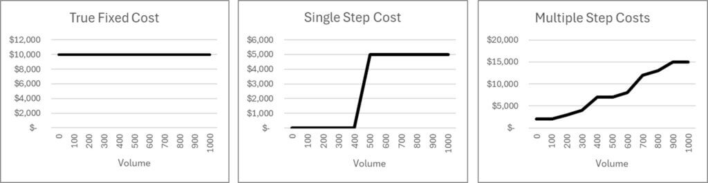
The preceding paragraphs are summarized in the three graphs below. The left graph shows a true fixed cost, as we assumed in earlier lessons. The middle graph is a single fixed cost, such as a new employee. The right graph represents the continuous increase in “fixed costs” as step costs are periodically added.
Getting the Bends
As British statistician George Box famously wrote, “All models are wrong; some are useful.” Revenues and costs in companies are rarely straight lines. However, CVP analysis using a straight line can be useful for modeling within a relevant range. As assumptions in the model move away from current amounts, we are less certain of the model’s accuracy.
Costs aren’t straight lines except over a small range of volume in real life. They bend. It’s important to know when bends are big. The key to identifying the bends is knowing capacity constraints and utilization. Managers can then decide whether to incur a big step cost to add capacity, which bends the cost line, or whether to cap production at current capacity.
Over a large range of volumes, the CVP line may be more curved than straight. How can we model this? Some math whiz types may try to find the formula for a curved line that best fits across a larger range of volume. The “bends” I’ve discussed may be so erratic that no single line fits the structure well.
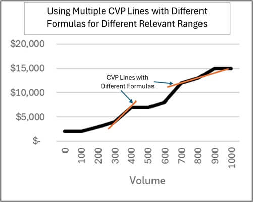
Another option is to use different CVP straight-line formulas at different volumes. You could think of these as tangent lines on a constantly curving CVP line. The difference between actual costs and that tangent line may be acceptably small over a short range of volumes on either side of the tangent point. Below is an example image with two CPV lines at different ranges of volumes with different formulas.
CVP and Marginal Profitability Analysis
CVP analysis and marginal profitability analysis are closely related. Marginal profitability analysis calculates the change in profit for a change in sales. The change in sales is often defined as one unit, but it can also be defined as any other number of units.
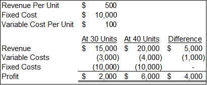
Below is a simple CVP and marginal profitability analysis. This models revenues and costs at 30 and 40 units. It’s the CVP formula calculation for both of them, but it can also be thought of as the marginal profit of going from 30 to 40 units. Over those ten units, revenues go up $5,000 (i.e., $500 X 10 units) and variable costs increase $1,000 (i.e., $100 X 10 units). Fixed costs don’t change over that range of production. Therefore, those fixed costs are not marginal costs.
CVP analysis captures all revenues and costs. Marginal profitability analysis is a much simpler analysis. We only need to know the costs and revenues that will change and how much they will change. All other costs and revenues are irrelevant.
Identifying and quantifying potential marginal costs is how we identify the bends in the CVP line that I discussed earlier. We can go to production managers and ask them whether they could produce ten more units, or whatever change we are modeling, with current resources or if they would need more. If they need more employees, we could then go to human resources, information technology, or other support departments to see if they would need more staff to support those employees. Costs lead to costs. In a large company with a wide range of revenues, each employee might feel more like a variable cost. In small companies, each employee feels more like a step cost.
When the marginal cost per unit is consistent across a range of units, then the contribution margin of CVP is the same as marginal profitability. You are within a relevant range for a single CVP formula. You are likely going beyond the boundary of the relevant range when there is a large change in marginal costs.
Check out my marginal profitability course if you want to learn more about marginal profitability analysis and its applications.
CVP and Uncertainty
The further volumes are from current volumes, the less certain we are about costs and revenues (and thus profit). That is why marginal contribution analysis as a change from current costs/revenues is most accurate; the starting numbers are best known.
In real life, most businesses are built incrementally. Rarely do companies have the opportunity to greatly increase sales. Each year, they grow revenues and costs incrementally (e.g., 10% growth per year). Many of them probably expected to be much more profitable at their current size when they were half their size, but found out there are many unknown costs along the way that pop up.
Incremental marginal analysis is good, but sometimes companies must step back and look strategically. What is the most profitable way for me to grow to be 10X my current size? This causes CVP to be modeled well past current volumes. Scenario analysis may be best when analyzing a specific desired state that’s far from the current state. It also allows layering in changes to many assumptions.
Another strategic question might be: Is higher profitability achievable at a smaller or larger size? Most companies grow incrementally to their current size and try to maximize revenue and cost for their current size. Another way to analyze a company is to break out its current sales into profitability layers. Rank all products by their contribution margin and identify the covariance of that margin with other products. Layer them in with different configurations to identify the fixed costs required for those volumes. Then, identify the highest profit scenario.
Companies shouldn’t grow past the point where their marginal returns are lower than the costs of capital (i.e., the alternative return owners could get with their cash). A company may have a much better return on equity (ROE) at a smaller size. You could calculate ROE at various sizes and determine when marginal ROE drops below the cost of capital or a similar hurdle rate.
In summary, the line drawn by CVP analysis visually overstates its precision, especially for volumes far from current volumes. One of my favorite quotes from the book Decisive by Chip and Dan Heath is, “The future isn’t a point; it’s a range.” As we’ve seen with the revenue and cost lines, the future is not a line; it’s a range. Sometimes, CVP analysis is a good modeling technique for exploring a path through the relevant range. Other modeling techniques may be better for exploring distant ranges.
For more info, check out these topics pages: