Warren Buffett once said, “Someone’s sitting in the shade today because someone planted a tree a long time ago.” In the same way, tomorrow’s profits may come from a strategy chosen from a decision tree you create today.
What is a Decision Tree?
A decision tree is a diagram that shows:
- Decisions to be made
- Uncertainties
- Potential outcomes
- The probability of each outcome
We saw the first two bullets in the influence diagram. Adding the second two bullets allows us to calculate the expected value (EV) of outcomes. Calculating the expected values helps us make the decision.
Benefits of a Decision Tree
Decision trees show the sequence of possibilities. Every path through the tree is a scenario for which we can calculate an expected value (EV).
The tree shows a range of outcomes, their probabilities, and the value of those outcomes. This helps us assess and clearly communicate both the EV and risk. We can better help evaluate the odds and severity of losing money or some other negative outcome.
Building a Decision Tree
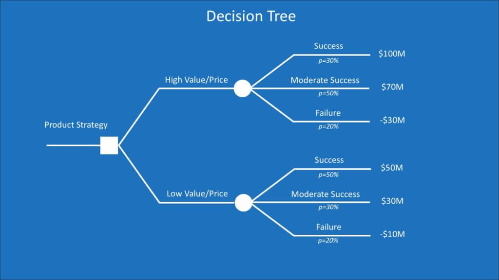
The image below is a decision tree for the product strategy decision discussed in the influence diagram lesson.
Let’s first look at the shapes in the diagram.
- Squares represent decisions. Our product strategy decision of introducing a high-price product or low-price product is the decision “root” of the tree.
- Circles are uncertainty nodes. Potential outcomes branch from those uncertainties. I show the probability of each outcome (e.g., p=30% for success for a high-price product) under each of those branches.
- The value of each outcome is a “leaf” on the tree. I’ve labeled each leaf with the NPV value of the outcome. You use whatever metric best measures what you value.
Like influence diagrams, the diagram flows chronologically from left to right. This reflects the order in which events will occur or uncertainties will be resolved. There are rules for the branches. The book Making Hard Decisions states that:
“Each [uncertainty] node must have branches that correspond to a set of mutually exclusive and collectively exhaustive outcomes. Mutually exclusive means that only one of the outcomes can happen… Collectively exhaustive means that no other possibilities exist; one of the specified outcomes has to occur. Putting these two specifications together means that when the uncertainty is resolved, one and only one of the outcomes occurs.”[1]
For you math fans, this means that the sum of the probabilities from an uncertainty node must add up to 100%.
I’ve simplified the outcomes to three options while there is a continuum of choices in reality. Thus, our choices can be thought of as representatives of ranges of that continuum. They can be thought of and analyzed as a discrete scenario or as a rough estimate EV of the range they represent.
In my example tree, the uncertain outcomes are qualitatively labeled “success,” “moderate success,” and “failure.” A big part of the decision team’s job is to clarify exactly what that means. In this case, it means mapping those subjective labels to discrete dollar amounts.
Calculating Expected Value
We now have the information we need to calculate expected values. Doing this via a decision tree is called “rolling back” or “folding back” the tree. This is because the calculations are done from right to left on the tree back toward our decision. We calculate values at each uncertainty node to find the EV to the right of the node. This ultimately leaves a set of EVs at the decision point from which we can select the one with the highest value. In complex trees, this is repeated for multiple sets of decisions and uncertainties.
Our simple tree had three potential outcomes from the decision to roll out a high-price product. They are summarized in this table:
| Outcome | Probability | NPV |
| Success | 30% | $100M |
| Moderate Success | 50% | $70M |
| Failure | 20% | -$30M |
To calculate the EV of the decision to roll out the high-price product, we calculate the weighted average EV of the outcomes. That is calculated as: (.30 X $100M) + (.50 X $70M) + (.20 X -$30M) = $59M.
The same logic is used for the low-price product. The EV calculation is: (.50 X $50M) + (.30 X $30M) + (.20 X -$10M) = $32M.
Our choice is now between a high-price product with an EV of $59M and a low-price product with an EV of $32M. This can be shown in a modified decision tree:
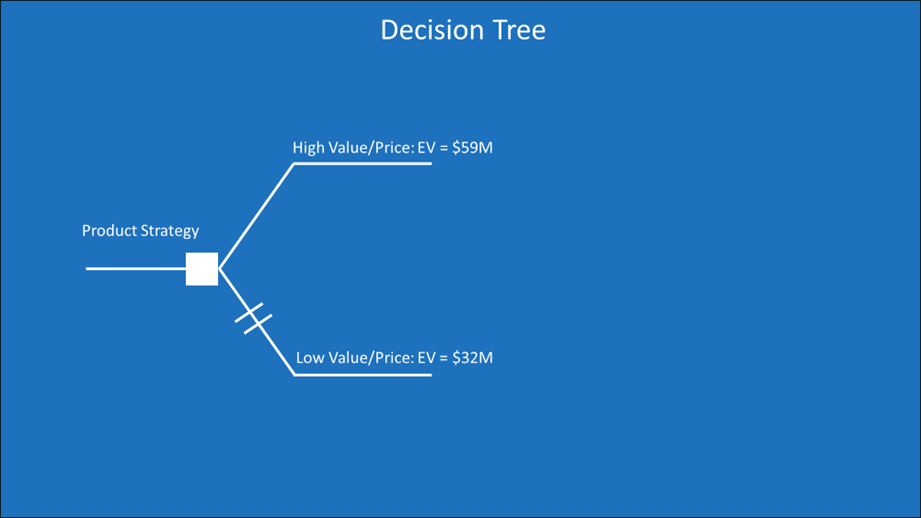
We choose the product with the highest EV. The option with the lower EV is shown with two lines cutting across it. We’ve “rolled back” the tree from 6 uncertain outcomes to the one branch at the decision point with the highest expected value. We’re pruning off poor uses of capital that lead to undesirable outcomes.
I live in Washington State, which produces the most apples of any state in the United States. The state produces around 7 billion tons of apples, which comprises 60% of U.S. apple production. You really should eat more apples. They are good for you and bring in billions of dollars to my state.
Apple growers prune a tree to maximize the tree’s energy available for producing the best fruit. Companies with limited time and resources must constantly make the same capital pruning decisions.
Decision Tree Software
There was a time not long ago when decision analysts wrote decision trees by hand and then barbarically rolled back that tree with slide rules or calculators. Modern technology saves us from such drudgery and the risk of errors.
It was easy to manually roll back our simple tree, but complex trees can be much trickier. And let’s face it: real-life decisions are complex.
There are Excel add-ins and standalone decision software that help you build and roll back a decision tree. You could manually create a decision tree to show your supervisor that buying this software is a good investment.
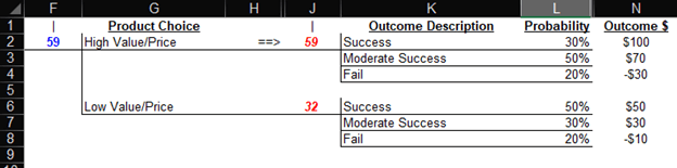
A free decision tree software named XLTree is available at https://www.probabilitymanagement.org/xltree. The image below shows the example tree from this course in XLTree.
Decision Trees and Influence Diagrams
Influence diagrams and decision trees can be used together to frame and make decisions. Each has different strengths in the decision-making process. Influence diagrams are a good way to initially frame the decision and develop relevant information. A decision tree is a good way to analyze and choose amongst key items from the influence diagram.
Decision trees better show the details of parts of the decision and how to evaluate them. However, the higher view of the influence diagram allows more to be considered.
Decision trees quickly get overwhelming when too much is considered for evaluation. The complexity of the tree rises geometrically with the number of uncertainties. This is why we only want to model the most important uncertainties in the tree.
Unimportant uncertainties can be considered on the influence diagram but don’t need to be carried over to the tree. Also, a work team may talk through a complex influence diagram but use a version with only the most important items for communication to decision-makers or implementation groups.
Influence diagrams are easier for people to understand. Decision trees are useful for explaining the choice in a decision once people understand the logic and calculation of a decision tree.
Decision Trees and Monte Carlo Simulation
Decision trees simplify a continuum of possibilities to a discreet set of outcomes. The outcomes from an uncertainty are often modeled as “yes/no” or “high/medium/low” options.
Monte Carlo simulation is a more comprehensive simulation analysis that utilizes a broader selection of possibilities and probabilities. It randomly picks from a range of assumptions over many iterations to create a range of potential outcomes. Probabilities for ranges in that continuum of outcomes can be calculated.
Decision trees assume a more deterministic (i.e., predictable pattern) of events, while Monte Carlo is more useful for stochastic (i.e., random and uncertain) analysis. Monte Carlo analysis can be very powerful, but it is more complex to create and communicate.
All models are simplifications of reality. The totality of reality is incomprehensible to all of us. It overwhelms decision-makers, even detail junkies like accountants and analysts. A decision tree is just a simplified proxy to represent the most relevant uncertainties in the forest of reality. Its simplification allows us to communicate, comprehend, consider, and calculate options.
As Oliver Wendell Holmes said, “For the simplicity on this side of complexity, I wouldn’t give you a fig. But for the simplicity on the other side of complexity, for that I would give you anything I have.”
The fear of simplification is that we’re missing something important. Monte Carlo simulation or other sensitivity analysis can be done on the uncertainties in our influence diagram to identify the most important to our decision. This can help us simplify without missing important items. Please see my course on sensitivity analysis to learn more about this.
Insights from Decision Trees
Now that we understand the structure of decision trees and how they help us calculate expected value, let’s look at some insights we can gain from them. Specifically, we’ll look at real options, break-even analysis, margin of safety, and risk.
The Value of Real Options
The example decision I used was between a high-price and a low-price product. Both products had the risk of loss. The high-price product had the highest EV but also the highest cost of failure.
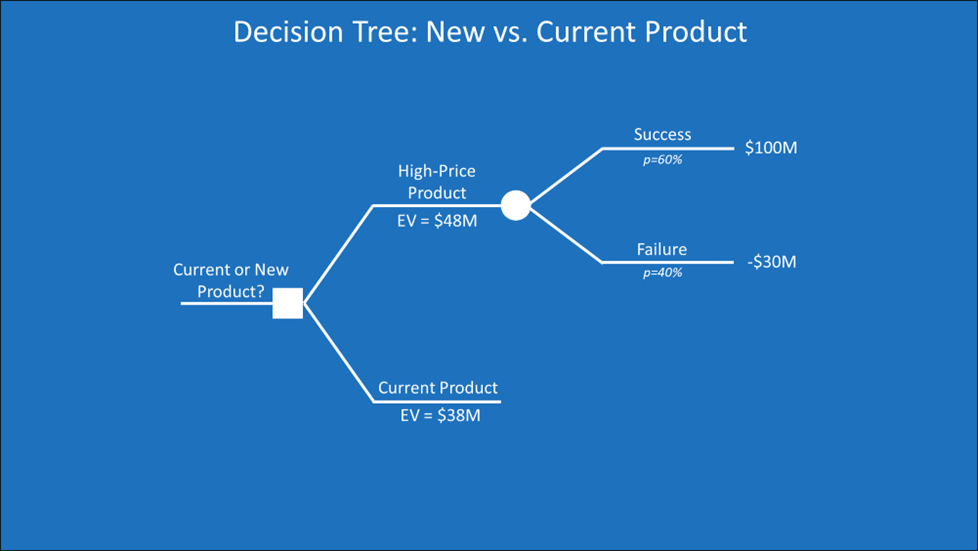
What if we had the option to test the market to obtain perfect information about whether the new high-price product will be a success? Below is a modification to the decision tree from our example.
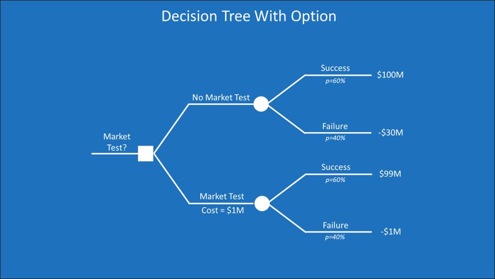
The decision on the left is now whether to market-test the new high-price product before rolling it out. Market testing costs $1M. I’ve simplified the outcome of the new product to a success with an NPV of $100M or a failure of -$30M. The probability of success is 60%.
The NPV of success if we do market testing is $99M, which is the $100M of NPV without testing, less the $1M of testing costs. The cost of failure if we test is only $1M. If the tests show that the product is a failure, we won’t roll out the new product, averting the $30M loss in the upper half of the diagram. You could add a decision not to roll out the product in both the upper and lower parts of the diagram.
Now, let’s roll back the tree. The EV of not testing the market is calculated as (.60 X $100M) + (.40 X -$30M) = $48M. The EV of testing is (.60 X $99M) + (.40 X -$1M) = $59M. The EV of market testing is $11M higher than not testing. We have a higher EV with less risk. We could make this example more complex by assuming that the information from the market testing is not certain and adding an uncertainty node for the probability that it gives us information that supports a bad decision.
This points to the importance of having options in decision-making and the value of information. Investopedia defines a real option as:
“An economically valuable right to make or else abandon some choice that is available to the managers of a company, often concerning business projects or investment opportunities. It is referred to as “real” because it typically references projects involving a tangible asset (such as machinery, land, and buildings, as well as inventory), instead of a financial instrument.”[2]
When we look at the uncertainties in an influence diagram and decision tree, we start to think about whether there is any way to reduce the uncertainty and what it’s worth to do so. Being able to eliminate the lowest NPV leaves of the tree can greatly improve our EV. Calculating the value of information gets into Bayesian logic that’s beyond this course, but it’s a course I will soon be releasing.
Using Decision Trees for Break-Even Analysis
Let’s look at another version of our decision tree.
The top part is the same as the last iteration. The bottom part is a simple branch for an existing product we have. This is a well-studied and stable current product of ours with an NPV of $38M. Our choice is to stay with our current product or replace it with a new high-price product.
The new high-price product has a higher EV than our current product, but this is subject to uncertain assumptions about the probability of success and the NPV if it’s a success. I picked those numbers out of the air. A real company might also pick numbers out of the air (calling it expert judgment) or may have done some analysis.
In a meeting to decide which product to go with, a huge amount of time may be wasted trying to decide whether 60% is the correct chance of success and whether the product will make $100M. There is a continuum of numbers the group can pick from and may debate about. It may be more efficient to turn the assessment of the assumptions into a yes/no question.
The yes/no question starts with these two questions:
- At what probability of success would the EV of the new product equal the EV of the current product?
- At what NPV would the EV of the new product equal the EV of the current product?
The formula for solving question #1 is:
(Probability of Success X $100M) + ((1- Probability of Success) X -$30M) = $38M
Using a little algebra magic, we find that the answer is roughly 52%, or 8% lower than our current estimate of 60%. We’re now ready for the yes/no question: Do we think that the probability of success is below 52%? If we do, the EV of the new product drops below that of the current product, so we should go with the current product (excluding any other information).
We can do the same for question #2. The formula for solving that is:
(.60 X NPV of Success) + (.4 X -$30M) = $38M
When we solve for the NPV of the Success, we determine that an NPV of $83M would equal an EV of $38M for the new product. Do we think that the NPV of a successful new product will be below $83M? If we do, the EV of the new product drops below that of the current product, so we should go with the current product (excluding any other information).
And for the Data Dogs out there that want to know the EVs of a mix of NPV and probabilities of success, here’s a two-variable data table for that:
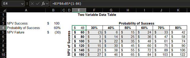
Each cell is an intersection of the EV of the new product at an NPV of success assumption and a probability of success assumption. The formula used for the EV calculation used in the table is at the top of the image. The cells shaded in grey (i.e., the cells in the top left half of the table) have EVs less than the $38M of the current product. For these mixes of assumptions, it’s likely better to go with the current product instead of rolling out the high-price product.
If you want to learn more about building break-even analyses and using two-variable data tables like above, check out my Cost-Volume-Profit (CVP) and Break-Even Analysis course.
EV and Risk
Decision trees are useful for measuring both expected value and risk. In our previous example, not everyone would choose the high-price product because it has the highest expected value. That choice also comes with a 40% probability of a $30 million loss.
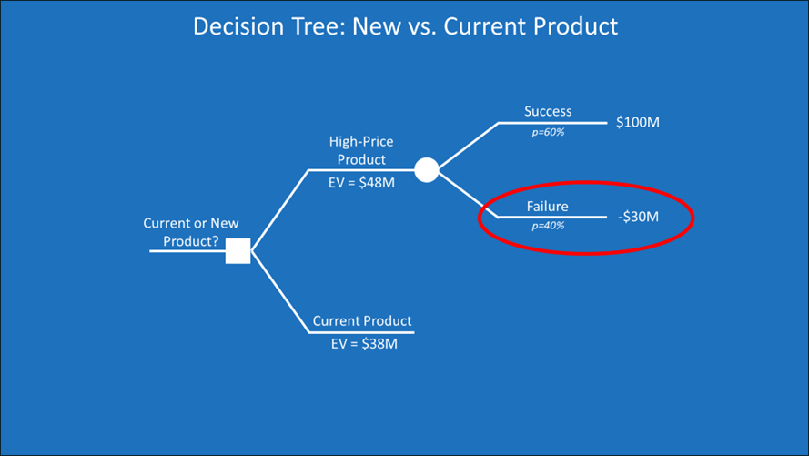
If I’m a mid-level manager in a big company and my whole job next year is the high-price product, I’m sweating buckets. There is an almost 50% chance my product will be an expensive failure, but company executives left the meeting expecting a $48M gain.
The CEO may have been comfortable with the $30 million loss because that loss will likely be offset by gains in other products. This is one reason to make decisions at a company portfolio level rather than looking at the expected value of projects one at a time in isolation.
The situation of a small-company CEO may be closer to the mid-level manager of a big company. A $30 million loss could bankrupt the company. I showed how real options are one option (pun intended) to reduce that risk. Financial options, like commodity futures, interest rate swaps, and currency hedges, are other ways that some companies mitigate the risk. A company that can’t handle the risk of an outcome of a leaf on the tree may have to cut off the whole branch.
Expected value assumes what’s called the law of large numbers. A flip of a coin has a 50% chance of landing heads and a 50% chance of landing tails. However, the outcome of one coin flip will be either 100% heads or 100% tails. The outcomes of a million coin flips may be closer to 50% heads and 50% tails. Business leaders are prone to overconfidence and an illusion of control. Bad outcomes get averaged into the good in the EV of the decision tree. Most decisions are about launching one product with one outcome, not launching a million products with an average result of those products. In other words, respect that any single decision can travel down any path of the tree and get the full outcome, not the EV.
The outcomes at the leaves of the tree, the probabilities of the branches, and the EV at the root decision are all important. The full decision tree shows all these amounts.
For more info, check out these topics pages:
[1] P. 74 of Making Hard Decisions by Clemen and Reilly
[2] https://www.investopedia.com/terms/r/realoption.asp