Estimating the change in profit of a price change requires an estimate of the price sensitivity of customers and the price-response function of a product.
Price Elasticity
Customer price sensitivity is the elasticity of demand you may have learned in economics. It’s not shocking that as the price of a product increases, the quantity purchased decreases. Lower prices increase the quantity purchased. The important assumption is how steep the slope of the demand line is. It was often shown with nifty graphs like this:
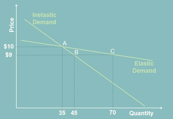
In this graph, a product is currently priced at $10. The market buys 35 of them. This is Point A in the image. The market price then drops to $9. How much will the quantity sold go up? The inelastic demand line has a steep slope. The quantity purchased only increases by ten units to a total of 45, which is Point B on the graph. Things are much different for the elastic demand line. The quantity purchased shoots up to 70 units.
What happens to profits for suppliers of the product? This can be summarized in a table.
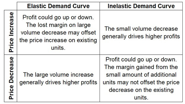
A price increase for a product with an elastic demand curve may cause an increase or a decrease in profit. The decrease in units sold may be so large that the lost margin on them is larger than the price increase from the rest of the units.
A similar dynamic occurs with a price decrease for a product with an inelastic demand curve. The additional margin from a small number of additional units may not be bigger than the sum of the decrease in price on the existing units. This is the danger of Point B in the previous image.
A price increase for a product with an inelastic demand curve and a price decrease for a product with an elastic demand curve both usually increase contribution to profit. Still, a price decrease that causes the margin per unit to be small to negative could cause profits to decrease for items with an elastic demand curve. A price increase at the far left (i.e., low quantities and high price) of an inelastic curve may cause a small decrease in units, but it’s a big percentage of sales and potential profits.
The takeaway so far is that a price increase or decrease can cause profit to go up or down, depending on the slope of the demand curve. If you know the demand curve, you can predict whether a price change is profitable.
There’s a problem. No one really knows the demand curve. Some price testing can help us estimate whether a price change is profitable, but I’ll talk about that later.
The Price-Response Function
The price-response function is similar to the elasticity of demand, except the price-response function specifies the demand for a product of a single seller as a function of price. The key difference is that the price-response function is for a single seller. Elasticity captures the dynamic of a market comprised of all sellers.
Why does the difference between the elasticity of demand and the price-response function matter? Different products and different companies have different price-response functions even though they are in the same market. Estimating the price-response function helps a company better project sales volumes at a new price, which is important for deciding whether to change prices. It’s difficult for a company to use industry data or even competitor sales to estimate the price-response function for their own product.
A company that reduces its price for a product may increase the overall customer demand for a product and/or take sales from other companies. As seen in this course, customers assess the price-volume trade-off of one product by comparing it to the price of a reference product plus the perceived net differentiation value.
The price-response function greatly changes when pricing is near competitors’ prices. Instead of the shape of the elasticity of demand curves, the price-response graph looks like this:
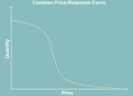
First, I want to point out that price and quantity have switched axes from the elasticity of demand graph. Price has moved to the x-axis. Quantity is on the y-axis. For whatever reason, elasticity of demand graphs and price-response graphs usually put price and quantity on opposite axes. It’s yet another way that very smart people confuse the rest of us. Now that we have our bearings, let’s look at what the graph tells us.
Pricing at the Three Sections of the Price-Response Graph
Let’s break the price-response graph into three sections titled A, B, and C. I’ll note pricing considerations for each section of the graph.
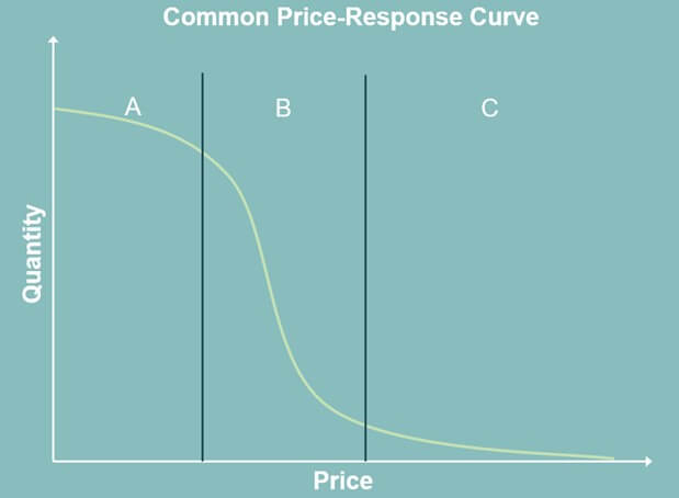
Section A
Prices are so low that few competitors exist. Companies must be very efficient to be profitable in this area. The price response is very low, so driving prices lower won’t likely drive large amounts of sales. At a certain price, further reductions are devastating to profits because they don’t drive enough volume to offset the price cannibalization. At an extreme, growth in volume doesn’t come from other companies but from attracting customers with a low willingness to pay into the market.
Section B
The middle part of the graph is very competitive. Small changes in price may cause large changes in volume. That assumes no one in the market changes their prices in response.
A reduction in price might be countered by one or more of the many competitors, so the price response is zero. Everyone makes less money. The lower prices might attract a few more buyers into the market via the elasticity of demand, but it likely won’t be enough to offset the price cannibalization. In this scenario, the whole curve slides to the left.
Section C
The right side of the graph is where companies that charge premium prices live. Through marketing and/or the perceived high value provided, they can demand high prices. The customers of these companies might be very loyal. They may find identity with a group or status by buying the company’s product, even at such a high price. Raising prices will cause little change in the quantity that’s sold.
What kills these products is when they are sucked into the middle of the graph. Competitors in the middle improve the value of their products. They build trust and loyalty with customers. If the premium competitor lowers their price in response, they lose much profit to cannibalization, so they don’t change their price until forced. However, these premium products often have high costs, either direct costs or indirect marketing and sales costs. They can’t be sold profitably when prices decrease, even when sales units increase as they are pulled into the middle of the market. Competitors with lower costs in the middle of the market then make higher profits and survive.
The Takeaways from the Price-Response Curve
The shape of the price-response curve greatly changes across big price changes. The range of the highest price response is where competition is fiercest. Expected large volume changes there could be negated by competitor price-matching.
There is a term in chess called “down-board thinking.” This means considering not just your next move but the array of your moves and competitor reactions over a few moves. Pricing requires the same thinking.
I’ll talk later about testing the price-response function. You may be able to estimate the volume changes from small price changes, absent competitor reactions. Extrapolating the volume changes from small changes in price to a large change in price is very difficult. In other words, a large price decrease or increase may not cause the change in sales units a company expects.
The Price-Response Curve for Individual Deals
The price-response graph line for low-priced products that are frequently purchased is closer to the smooth line graph I just talked about. Pricing for these is usually set with list prices set by a committee, department, or team.
Large-dollar purchases made infrequently have a very different graph. At an extreme, it looks like the image below.
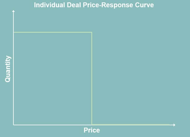
Either you get the deal, or you don’t. In those cases, you might have to use historical bid history to inform pricing, but it will take expert opinions from either a single salesperson or a group to determine the bid price.
Narrow framing limits one’s vision to each decision. Broad framing sees each decision in the context of other decisions. Broad framing judges the performance of a group of decisions as a whole.
Narrow framing puts great pressure on getting each deal. This causes sellers to be risk-averse to losing the deal, which leads to lower pricing. The focus becomes pricing tactics. Price cuts and discounts become very tempting.
A broad-frame view changes the focus from tactics to strategy. The pricing-response curve is perceived as the smooth curve pictured earlier. You win some deals and lose some deals, but the pricing strategy holds you at the optimum price at a minimum expected volume over the long term. If the projected volume at that price looks like it won’t be achieved over the long term, then the strategy needs to be adjusted. Sales goals and commissions for individual performance versus team-based or profit-based incentives may detract from broad-view thinking.
Ways to Estimate the Price-Response Function
There are many ways to estimate the price response of customers. They can generally be broken into data based on actual purchases and data based on customer-stated preferences. They include analyzing purchase data, surveys, interviews, purchase experiments, and conjoint analysis.
It’s amazing how far some companies go, including creating simulation stores that people shop in. Most of this is marketing analysis that’s beyond the scope of this course. I did want to touch briefly on some quantitative techniques.
Historical Sales and Price Tracking
The first is historical sales tracking. Sales at an aggregate or at the product level can provide a wealth of information. Focus on product volumes before and after a price change by your company or by a competitor. This can provide data about the price-response function for that product.
Let’s assume a company was charging $30 for a product and then increased the price to $33. Their sales went from 20,000 units to 16,000 units. Their costs were $22 per unit. Was this a profitable price increase?
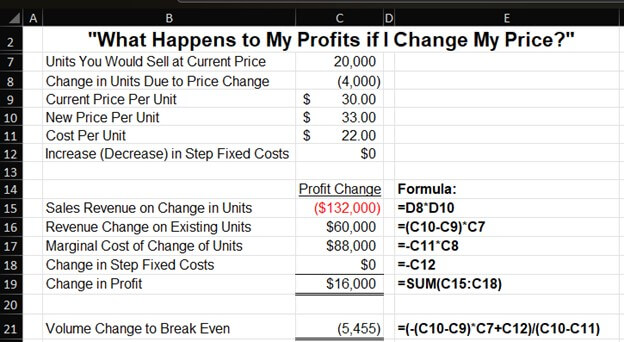
The answer is yes. If managers only looked at revenue, they may have been worried about the $72,000 drop in revenue (the sum of cells C15 and C16). This was more than offset by the decrease in production costs. The breakeven analysis shows that sales could have dropped 5,455 units before the company lost money on the price increase.
A price change can be made with one large change or through a series of smaller changes. One large change allows faster feedback across two very different price points. The problem with this is that the new price may be disastrous, and its negative effects may take some time to undo. Making repeated small changes combined with constant monitoring takes longer, but a company may find an optimal point as it keeps changing prices.
A/B Testing
A/B testing is trying different prices for the same product or similar products. In pure A/B testing, people are randomly assigned different offers. For example, a website might show different pages to different people at the same time.
There are some dangers with this. There are stories of people who went to the same website multiple times in a short amount of time and received different prices. These people had reduced trust in the vendor and talked about it on social media.
A company must be very careful not to appear unfair on who gets the higher and lower pricing. Some variations on A/B testing to consider include:
- Testing different prices in different markets
- Change the price over a short period of time with frequent monitoring
- Have two very slightly different products with different prices
- Start with a list price and offer varying discounts
A/B testing can be more accurate than historical sales tracking because the testing of different price points is concurrent. Sales volumes tracked over time can vary for many reasons aside from the price change. However, not all products can be concurrently differently priced via A/B testing.
Win/Lose Tracking
For products priced via bids, a company can track the prices of the deals they got versus the ones they didn’t get. This helps build data points for analyzing the price sensitivity of customers. In other words, what is the general likelihood of getting a deal at a given price? If we lower the price, how much does the probability of a sale go up? Do the higher win rates compensate for the reduced prices?
Here’s a simplified example. The table below shows whether a company won or lost various bids grouped into price bands.
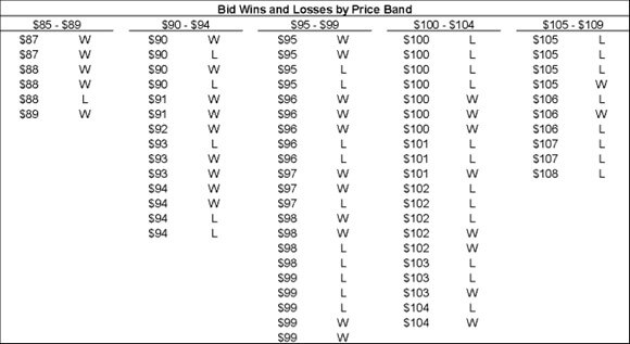
You can then calculate the percentage of bids that were won or lost by price band:
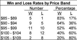
Those percentages are source information about the price-response function. The probability of a win can be multiplied by the gross margin of a sale to arrive at a probability-weighted margin. The following table multiples the margin times the probability of winning a bid at varying costs, prices, and margins.
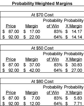
At a $70 cost, the probability-weighted margins are very similar. At a $50 cost, the probability-weighted margin is better for the lower $87 price. The opposite is true when costs per unit are $80.
Once again, this is just one piece of information for analyzing the profitability or pricing. You can layer in other concepts from my pricing courses, like price cannibalization rates. The profitability would be very different depending on whether the product costs above are sunk costs or truly marginal costs.
This analysis looks at the relationship between price and win rates. There may be many other factors that influence win rates. There are variations in customers, products, and market conditions that influence win rates.
One note of caution is that two bids at the same price could have vastly different probabilities of leading to a sale because of how each customer is using the bid. A customer may just be getting bids to force their favorite vendor to reduce prices.
Data and Interpretation
The results from all these methods will require interpretation. It’s always amazing how people can look at the same data and develop different stories from it. None of these methods provide perfectly controlled experiments. The economy, customer preferences, and competitors are always changing. The data is only a starting point with which managers make qualitative analyses to set pricing strategies and tactics.
For more info, check out these topics pages: